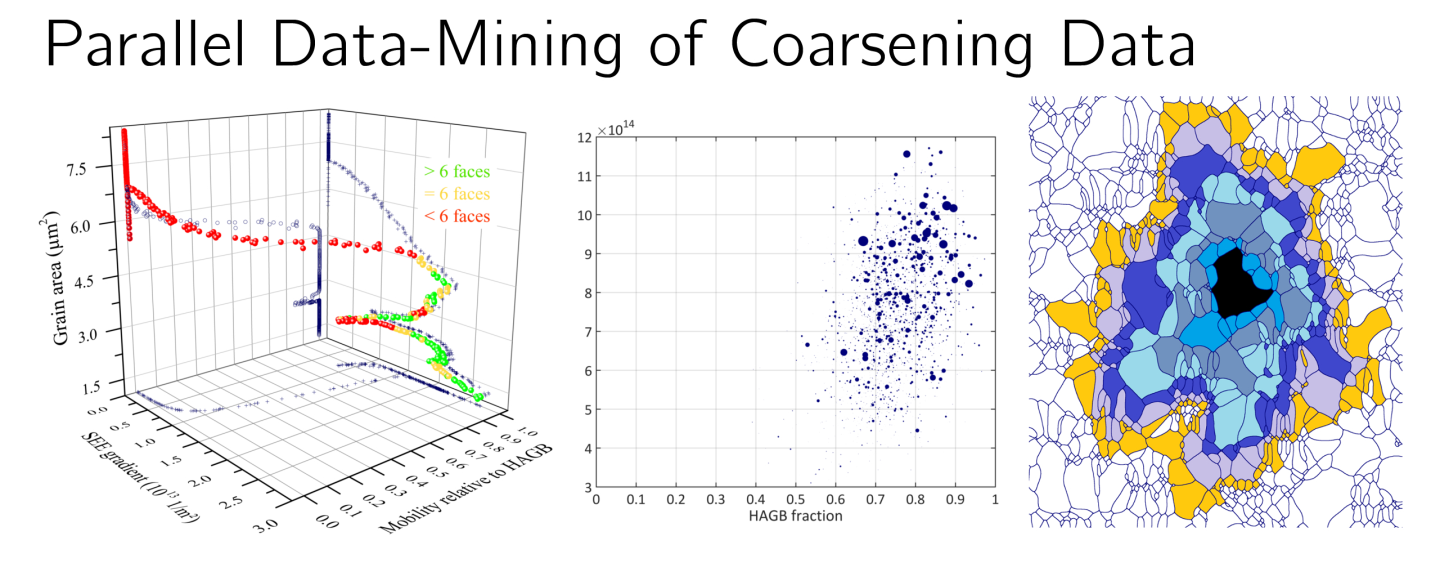
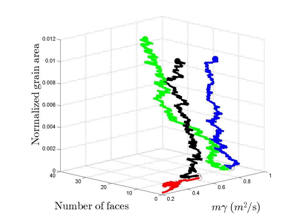
TopologyTracer is an MPI/OpenMP-parallelized datamining tool for conducting spatio-temporal analyses of microstructural element dynamics. Its purpose is the quantification of correlations — spatial and temporal — between individual microstructural elements and their higher-order neighboring elements. Currently, the software allows comprehensive studies of individual grains’ volume evolution and set their growth history into relation to the evolution of their higher-order neighbors. The tool is unique in two ways: on the one hand in its ability to process these surveys in parallel and thereby handle hitherto intractable large datasets including millions of grains. On the other hand in its capability to explicitly take the spatial distribution of the long range neighborhood into account.

The source code was developed by Markus Kühbach during his PhD time with Luis A. Barrales-Mora and Günter Gottstein at the Institute of Physical Metallurgy and Metal Physics (IMM) with RWTH Aachen University. Being now with the Max-Planck-Institut fur Eisenforschung GmbH in Düsseldorf, I maintain the code, though at disregular intervals. Nonetheless, feel free to utilize the tool, do not hesitate contacting me for sharing thoughts, suggesting improvements, or reporting your experiences.

1. Getting started

• In a nutshell
  • What is the TopologyTracer?
  • What are the user benefits?
  • What sets the TopologyTracer apart from other tools like DREAM3D or MTex?
• References
  • The method
  • Contact
  • Specifically about GraGLeS
  • Third-party contributions
• Setup
  • Which prerequisites are necessary?
  • Which prerequisites are optional?
  • Where to get source code from?
  • Placement of files
  • Optimization
  • Troubleshooting?!

2. Creating input

• What is TopologyTracer input?
• Binary file format layout
  • Grain boundary face data via Faces files
  • Grain meta data via Texture files
  • Illustrative example of expected datavolume

3. TopologyTracing

TopologyTracing requires at least to have

1. A collection of ID contiguous binary data file pairs, i.e. Faces_*.bin and Texture_*.bin binary files,
2. The topotracer2d3d executable,
3. A XML control file all in the same folder.

Several analysis routines require additional files as it is explained for many in the input section.

With these prerequisites, TopologyTracing, i.e. the datamining of simulation data, requires two steps:

1. Setup the control file

2. Specify the post-processing tasks

Both tasks are accomplished via the XML control file:

• XML Control File Settings
  • Analysis mode
  • Fundamental settings
  • Physical properties
  • Datamining operations
  • Datamining operation specific settings
  • Auxiliary files
  • Additional settings
• Program execution
  • MPI only
  • MPI/OpenMP
• Compile a growth history for individual grains
• Output data format specification
  • analyze_vol_quantiles()
  • analyze_vol_forward()
  • analyze_vol_backward()
  • analyze_sizegain_vs_bk()
  • analyze_approx_rxfraction()
  • analyze_modf()
  • analyze_see()
  • analyze_gsd()
  • analyze_abnormal_graingrowth()
  • Currently undocumented

4. Visualizing results

In its current state, the TopologyTracer does not contain a GUI. Instead, plain MPI I/O raw files and ASCII files are generated which require post-processing with for instance Matlab scripts available in the scripts folder. In general one can visualize a growth path by the plot3(X,Y,Z) command and access a distribution of values via the histogram function. Therein X, Y, Z specify each a row vector of length NC for a particular grain ID in row r.

Funding

The authors gratefully acknowledge the support from the DFG in the frame of the Reinhart Koselleck project (GO 335/44-1).

Furthermore, we acknowledge the support from the FZJülich and RWTH Aachen University within the JARAHPC research alliance.

In addition I would like to acknowledge the provision of computing resources by the Max Planck-Institut für Eisenforschung GmbH.

Version history

v1.2

Implementation of tracking mode 2 which does not require any longer the entire dataset to be loaded in main memory, but

instead reads successively files for analyses. This patch makes the program also applicable to low main memory workstations.

Implementation of 3D extension to unbiased longer range environment measures via Monte Carlo sampling,

curvature estimation via binary contour line data single-grain-resolved for arbitrary number of time steps,

binning of stored elastic energy in grain population, tracking of maximum size of grain during its existence.

Bug fixing, implementation of allocation error handling, performance updates in particular beneficial for handling

hundred thousand grain ID long lists of candidate grains for population categorization.

Clean-up of source code debris and documentation of cmake script.

Clean-up of and provision of Matlab-based analysis scripts for post-processing and their core documentation.

v1.0

Successful switch from ASCII- to binary file-based workflow, locality-aware data organization, and tree-based

data storage improved raw data I/O by orders of magnitude. Furthermore, it made collecting random grain properties

orders of magnitude more efficient. Novel algorithm to identify k-th order neighbors makes now possible the tracking

of arbitrary k-th order neighbors. Novel analysis routines make possible the comparison to classical theory of abnormal grain

growth and classical nucleation criteria (Bailey-Hirsch, sub-grain size distribution spreading to name but a few).

Additionally, the code supports now functionality to compute analytically the triangle-circle intersection area.

v0.1

Implementation of first set of functionalities to obtain temporal trajectories in topology/mobility/energy-phase space for the Riso 2015 conference with simple neighbor correlations and disorientation.

Licence

• The project is licenced under the GNU v3.0

Questions, contributions

Just let me know or contact m.kuehbach@mpie.de

Future plans

v1.3

Documentation, 3D curvature computation, triple line tracking